Estimate power analysis for choice experiment designs

This function estimates the same model multiple times using different sample sizes to assess statistical power. It returns both the estimated models and a summary of coefficient estimates, standard errors, and power statistics.

Usage

cbc_power(
  data,
  outcome = "choice",
  obsID = "obsID",
  pars = NULL,
  randPars = NULL,
  n_breaks = 10,
  n_q = NULL,
  panelID = NULL,
  alpha = 0.05,
  return_models = FALSE,
  n_cores = NULL,
  ...
)

Arguments

data: A data frame containing choice data. Can be a cbc_choices object or any data frame with the required columns.
outcome: Name of the outcome variable column (1 for chosen, 0 for not). Defaults to "choice".
obsID: Name of the observation ID column. Defaults to "obsID".
pars: Names of the parameters to estimate. If NULL (default), will auto-detect from column names for cbc_choices objects.
randPars: Named vector of random parameters and their distributions ('n' for normal, 'ln' for log-normal). Defaults to NULL.
n_breaks: Number of sample size groups to test. Defaults to 10.
n_q: Number of questions per respondent. Auto-detected for cbc_choices objects if not specified.
panelID: Name of the panel ID column for panel data. Auto-detected as "respID" for multi-respondent cbc_choices objects.
alpha: Significance level for power calculations. Defaults to 0.05.
return_models: If TRUE, includes full model objects in returned list. Defaults to FALSE.
n_cores: Number of cores for parallel processing. Defaults to parallel::detectCores() - 1.
...: Additional arguments passed to logitr::logitr().

Value

A cbc_power object containing:

power_summary: Data frame with sample sizes, coefficients, estimates, standard errors, t-statistics, and power
models: List of estimated models (if return_models = TRUE)
sample_sizes: Vector of sample sizes tested
n_breaks: Number of breaks used
alpha: Significance level used

Examples

library(cbcTools)

# Create profiles and design
profiles <- cbc_profiles(
  price = c(1, 2, 3),
  type = c("A", "B", "C"),
  quality = c("Low", "High")
)

design <- cbc_design(profiles, n_alts = 2, n_q = 6)

# Simulate choices
priors <- cbc_priors(profiles, price = -0.1, type = c(0.5, 0.2), quality = 0.3)
choices <- cbc_choices(design, priors)

# Run power analysis
power_results <- cbc_power(choices, n_breaks = 8)
#> Auto-detected parameters: price, typeB, typeC, qualityHigh
#> Using 'respID' as panelID for panel data estimation.
#> Estimating models using 3 cores...
#> Model estimation complete!

# View results
print(power_results)
#> CBC Power Analysis Results
#> ==========================
#> 
#> Sample sizes tested: 12 to 100 (8 breaks)
#> Significance level: 0.050
#> Parameters: price, typeB, typeC, qualityHigh
#> 
#> Power summary (probability of detecting true effect):
#> 
#> n = 12:
#>   price       : Power = 0.234, SE = 0.2189
#>   typeB       : Power = 0.476, SE = 0.5480
#>   typeC       : Power = 0.375, SE = 0.5332
#>   qualityHigh : Power = 0.131, SE = 0.3701
#> 
#> n = 38:
#>   price       : Power = 0.056, SE = 0.1161
#>   typeB       : Power = 0.051, SE = 0.2393
#>   typeC       : Power = 0.138, SE = 0.2326
#>   qualityHigh : Power = 0.870, SE = 0.1928
#> 
#> n = 50:
#>   price       : Power = 0.104, SE = 0.0977
#>   typeB       : Power = 0.185, SE = 0.2054
#>   typeC       : Power = 0.052, SE = 0.1999
#>   qualityHigh : Power = 0.773, SE = 0.1696
#> 
#> n = 75:
#>   price       : Power = 0.178, SE = 0.0820
#>   typeB       : Power = 0.869, SE = 0.1677
#>   typeC       : Power = 0.188, SE = 0.1644
#>   qualityHigh : Power = 0.876, SE = 0.1359
#> 
#> n = 100:
#>   price       : Power = 0.121, SE = 0.0712
#>   typeB       : Power = 0.914, SE = 0.1451
#>   typeC       : Power = 0.084, SE = 0.1423
#>   qualityHigh : Power = 0.989, SE = 0.1165
#> 
#> Use plot() to visualize power curves.
#> Use summary() for detailed power analysis.
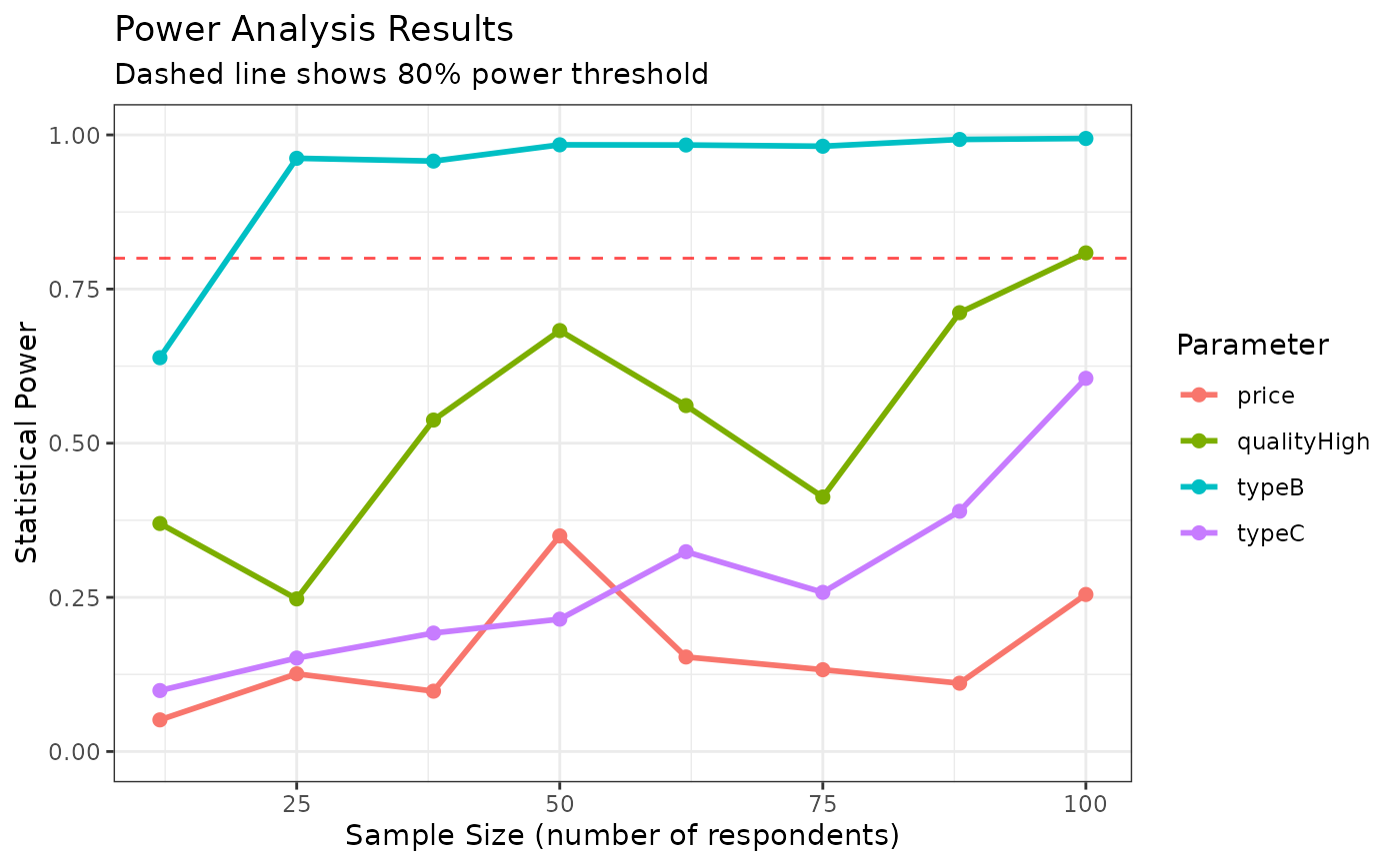
plot(power_results)