Getting Started
Learning Objectives
- Get familiar with using R in RStudio
- Create and store values as objects.
- Be able to use R as a calculator.
- Know some of the ways R handles certain things, like spaces.
- Know how to create comments with the
#symbol.- Be able to compare values in R.
- Know some common functions in R.
- Know how R handles function arguments and named arguments.
- Know how to install, load, and use functions from external R packages.
- Know some best practices for staying organized in R with R projects.
1 R and RStudio
R is a programming language that runs computations, and RStudio is an interface for working with R with a lot of convenient tools and features. It is the primary integrated development environment (IDE) for R users.
You can think of the two like this:
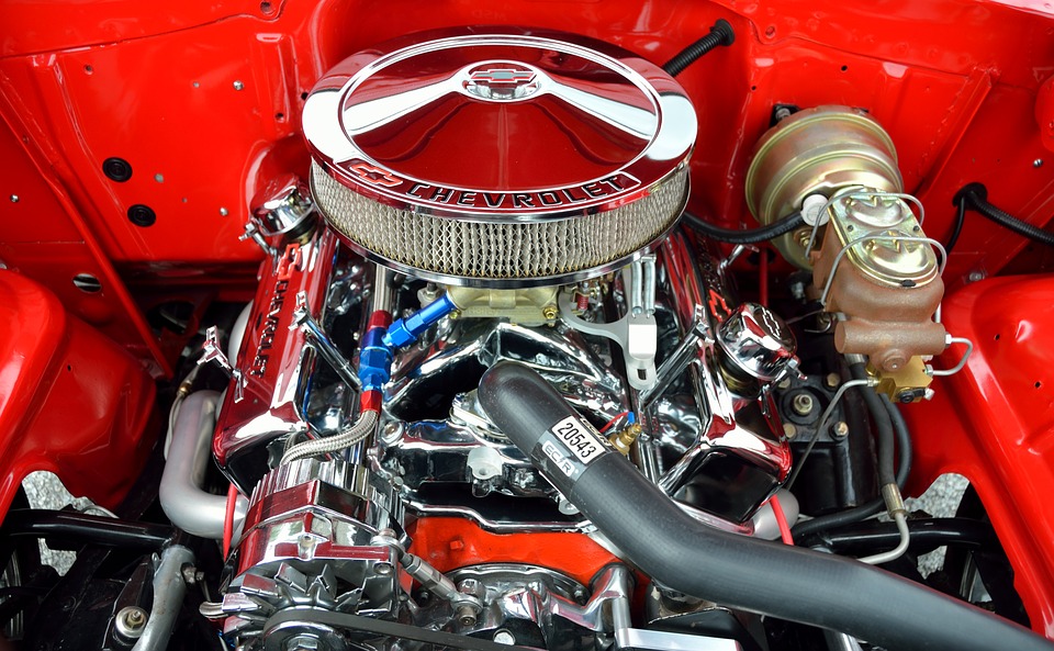
- R is like a car’s engine.
- RStudio is like a car’s dashboard.
| R: Engine | RStudio: Dashboard |
|---|---|
 |
 |
Your car needs an engine (R) to run, but having a speedometer and rear view mirrors (RStudio) makes driving a lot easier.
To get started using R , you need to download and install both R and RStudio (Desktop version) on your computer. Go to the course prep page for instructions.
Once you have everything installed, open RStudio. You should see the following:
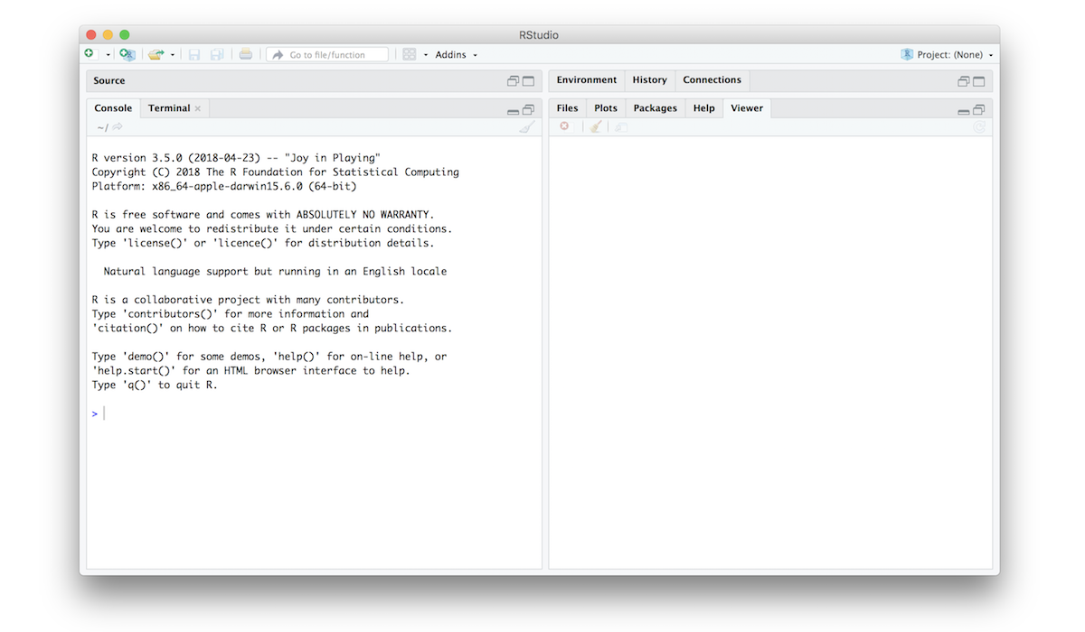
Notice the default panes:
- Console (entire left)
- Environment/History (tabbed in upper right)
- Files/Plots/Packages/Help (tabbed in lower right)
FYI: you can change the default location of the panes, among many other things: Customizing RStudio.
Go into the Console on the left with the > (that’s
the command prompt).
Let’s get started using R!
2 Your first conveRsation
When you type something into the console, R will give you a reply. Think of it like having a conversation with R. For example, let’s ask R to add two numbers:
3 + 4## [1] 7As you probably expected, R returned 7. No surprises
here!
Quick note: you can ignore the
[1]you see in the returned value…that’s just R saying there’s only one value to return.
But what happens if you ask R to add a number surrounded by quotations marks?
3 + "4"## Error in 3 + "4": non-numeric argument to binary operatorLooks like R didn’t like that. That’s because you asked R to add a
number to something that is not a number ("4" is a
character, which is different from the number 4),
so R returned an error message. This is R’s what of telling you that you
asked it to do something that it can’t do.
Here’s a helpful tip:
EMBRACE THE ERROR MESSAGES!
By the end of this course, you will have seen loads of error messages. This doesn’t mean you “can’t code” or that you’re “bad at coding” - it just means you’ve still got more work to do to solve the problem.
In fact, the best coders sometimes intentionally write code with known errors in it in order to get an error message. This is because when R gives you an error message, most of the time there is a hint in it that can help you solve the problem that led to the error. For example, take a look at the error message from the last example:
Error in 3 + "4" : non-numeric argument to binary operatorHere R is saying that there was a “non-numeric argument” somewhere.
That suggests that the problem might be with something not being a
number. As we just discussed, "4" is a character, or a
“non-numeric argument”.
With practice, you’ll get better at embracing and interpreting R’s error messages.
3 Storing values
You can store values by “assigning” them to an object with
the <- symbol, like this:
x <- 2Here the symbol <- is meant to look like an arrow. It
means “assign the value 2 to the object named
x”.
PRO TIP: To quickly type
<-, use the shortcutoption+-(mac) oralt+-(windows). There are lots of other helpful shortcuts. TypeAlt+Shift+Kto bring up a shortcut reference card).
Since we assigned the value 2 to x, if we
type x into the console and press “enter” R will return the
stored value:
x## [1] 2If you overwrite an object with a different value, R will “forget” the previous assigned value and only keep the new assignment:
x <- 42
x
## [1] 42PRO TIP: Always surround
<-with spaces to avoid confusion! For example, if you typedx<-2(no spaces), it’s not clear if you meantx <- 2orx < -2. The first one assigns2tox, but the second one compares whetherxis less than-2.
3.1 Use meaningful variable names
You can choose almost any name you like for an object, so long as the
name does not begin with a number or a special character like
+, -, *, /,
^, !, @, or &.
But you should always use variable names that describe the thing
you’re assigning. This practice will save you major headaches
later when you have lots of objects in your environment.
For example, let’s say you have measured the length of a caterpillar and want to store it as an object. Here are three options for creating the object:
Poor variable name:
x <- 42Good variable name:
length_mm <- 42Even better variable name:
caterpillar_length_mm <- 42The first name, x, tells us nothing about what the value
42 means (are we counting something? 42 of
what?). The second name, length_mm, tells us that
42 is the length of something, and that it’s measured in
millimeters. Finally, the last name, caterpillar_length_mm,
tells us that 42 is the length of a caterpillar, measured
in millimeters.
3.2 Use standard casing styles
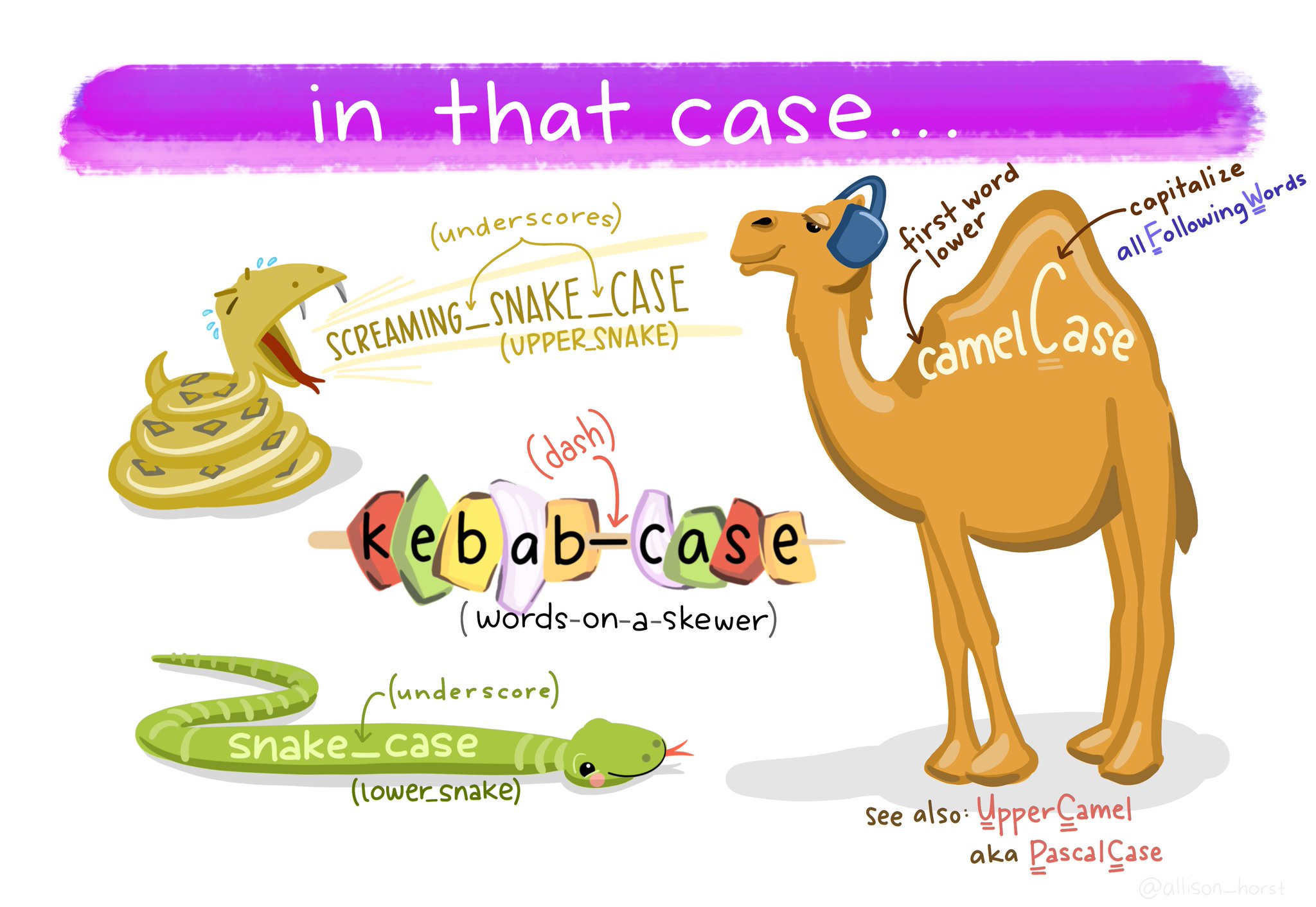 Art by Allison
Horst
Art by Allison
Horst
You will be wise to adopt a convention for demarcating words in names. I recommend using one of these:
snake_case_uses_underscorescamelCaseUsesCaps
Make another assignment:
this_is_a_long_name <- 2.5To inspect this, try out RStudio’s completion facility: type the first few characters, press TAB - voila! RStudio auto-completes the long name for you :)
3.3 R is case sensitive
To understand what this means, try this:
cases_matter <- 2
Cases_matter <- 3
Let’s try to inspect:
cases_matter## [1] 2Cases_matter## [1] 3Although the two objects look_ similar, one has a capital “C”, and R stores that as a different object.
In general, type carefully. Typos matter. Case matters. Get better at typing.
3.4 The workspace
Look at your workspace in the upper-right pane. The workspace is where user-defined objects accumulate. You can also get a listing of these objects with commands:
objects()## [1] "cases_matter" "Cases_matter" "caterpillar_length_mm"
## [4] "length_mm" "this_is_a_long_name" "x"ls()## [1] "cases_matter" "Cases_matter" "caterpillar_length_mm"
## [4] "length_mm" "this_is_a_long_name" "x"If you want to remove the object named x, you can do
this
rm(x)To remove everything, use this:
rm(list = ls())or click the broom symbol.
4 R as a calculator
4.1 Arithmetic operators
You can do a ton of things with R, but at its core it’s basically a fancy calculator. R handles simple arithmetic using the following arithmetic operators:
| operation | operator | example input | example output |
|---|---|---|---|
| addition | + |
10 + 2 |
12 |
| subtraction | - |
9 - 3 |
6 |
| multiplication | * |
5 * 5 |
25 |
| division | / |
9 / 3 |
3 |
| power | ^ |
5 ^ 2 |
25 |
The first four basic operators (+, -,
*, /) are pretty straightforward and behave as
expected:
7 + 5 # Addition## [1] 127 - 5 # Subtraction## [1] 27 * 5 # Multiplication## [1] 357 / 5 # Division## [1] 1.4Not a lot of surprises (you can ignore the [1] you see
in the returned values…that’s just R saying there’s only one value to
return). Powers are represented using the ^ symbol. For
example, to calculate \(5^4\) in R, we
would type:
5^4## [1] 6254.2 Order of operations
R follows the typical BEDMAS order of operations. That is, R evaluates statements in this order1:
- Brackets
- Exponents
- Division
- Multiplication
- Addition
- Subtraction
For example, if I type:
1 + 2 * 4## [1] 9R first computes 2 * 4 and then adds 1. If
what you actually wanted was for R to first add 2 to
1, then you should have added parentheses around
1 and 2:
(1 + 2) * 4## [1] 12A helpful rule of thumb to remember is that brackets always come first. So, if you’re ever unsure about what order R will do things in, an easy solution is to enclose the thing you want it to do first in brackets.
4.3 R ignores excess spacing
When I typed 3 + 4 before, I could equally have done
this
3 + 4## [1] 7or this
3 + 4## [1] 7Both produce the same result. The point here is that R ignores extra spaces. This may seem irrelevant for now, but in some programming languages (e.g. Python) blank spaces matter a lot!
This doesn’t mean extra spaces never matter. For example, if
you wanted to input the value 3.14 but you put a space
after the 3, you’ll get an error:
3 .14## Error: <text>:1:5: unexpected numeric constant
## 1: 3 .14
## ^Basically, you can put spaces between different values, and you can put as many as you want and R won’t care. But if you break a value up with a space, R will send an error message.
4.4 Using comments
In R, the # symbol is a special symbol that denotes a
comment. R will ignore anything on the same line that follows the
# symbol. This enables us to write comments around our code
to explain what we’re doing:
speed <- 55 # This is km/h, not mph!
speed
## [1] 55Notice that R ignores the whole sentence after the #
symbol.
5 Comparing things
Other than simple arithmetic, another common programming task is to compare different values to see if one is greater than, less than, or equal to the other. R handles comparisons with relational and logical operators.
5.1 Comparing two things
To compare two things, use the following relational operators:
- Less than:
< - Less than or equal to :
<= - Greater than or equal to:
>= - Greater than:
> - Equal:
== - Not equal:
!=
The less than operator < can be used to test
whether one number is smaller than another number:
2 < 5## [1] TRUEIf the two values are equal, the < operator will
return FALSE, while the <= operator will
return TRUE: :
2 < 2## [1] FALSE2 <= 2## [1] TRUEThe “greater than” (>) and “greater than or equal to”
(>=) operators work the same way but in reverse:
2 > 5## [1] FALSE2 > 2## [1] FALSE2 >= 2## [1] TRUETo assess whether two values are equal, we have to use a double equal
sign (==):
(2 + 2) == 4## [1] TRUE(2 + 2) == 5## [1] FALSETo assess whether two values are not equal, we have to use
an exclamation point sign with an equal sign (!=):
(2 + 2) != 4## [1] FALSE(2 + 2) != 5## [1] TRUEIt’s worth noting that you can also apply equality operations to
“strings,” which is the general word to describe character values
(i.e. not numbers). For example, R understands that a
"penguin" is a "penguin" so you get this:
"penguin" == "penguin"## [1] TRUEHowever, R is very particular about what counts as equality. For two pieces of text to be equal, they must be precisely the same:
"penguin" == "PENGUIN" # FALSE because the case is different## [1] FALSE"penguin" == "p e n g u i n" # FALSE because the spacing is different## [1] FALSE"penguin" == "penguin " # FALSE because there's an extra space on the second string## [1] FALSE5.2 Making multiple comparisons
To make a more complex comparison of more than just two things, use the following logical operators:
- And:
& - Or:
| - Not:
!
And:
A logical expression x & y is TRUE only
if both x and y are
TRUE.
(2 == 2) & (2 == 3) # FALSE because the second comparison if not TRUE## [1] FALSE(2 == 2) & (3 == 3) # TRUE because both comparisons are TRUE## [1] TRUEOr:
A logical expression x | y is TRUE if
either x or y are
TRUE.
(2 == 2) | (2 == 3) # TRUE because the first comparison is TRUE## [1] TRUENot:
The ! operator behaves like the word “not” in
everyday language. If a statement is “not true”, then it must be
“false”. Perhaps the simplest example is
!TRUE## [1] FALSEIt is good practice to include parentheses to clarify the statement or comparison being made. Consider the following example:
!3 == 5## [1] TRUEThis returns TRUE, but it’s a bit confusing. Reading
from left to right, you start by saying “not 3”…what does that mean?
What is really going on here is R first evaluates whether 3 is equal
to 5 (3 == 5), and then returns the “not” (!)
of that. A better version of the same thing would be:
!(3 == 5)## [1] TRUE6 Functions
To do more advanced calculations you’re going to need to start using functions.
R has a lot of very useful built-in functions. For example, if I
wanted to take the square root of 225, I could use R’s built-in square
root function sqrt():
sqrt(225)## [1] 15Here the letters sqrt are short for “square root,” and
the value inside the () is the “argument” to the function.
In the example above, the value 225 is the “argument”. Keep
in mind that not all functions have (or require) arguments:
date() # Returns the current date and time## [1] "Mon Sep 4 20:01:01 2023"(the date above is the date this page was last built)
6.1 Frequently used functions
R has LOTS of functions. Many of the basic math functions are somewhat self-explanatory, but it can be hard to remember the specific function name. Below is a reference table of some frequently used math functions.
| Function | Description | Example input | Example output |
|---|---|---|---|
round(x, digits=0) |
Round x to the digits decimal place |
round(3.1415, digits=2) |
3.14 |
floor(x) |
Round x down the nearest integer |
floor(3.1415) |
3 |
ceiling(x) |
Round x up the nearest integer |
ceiling(3.1415) |
4 |
abs() |
Absolute value | abs(-42) |
42 |
min() |
Minimum value | min(1, 2, 3) |
1 |
max() |
Maximum value | max(1, 2, 3) |
3 |
sqrt() |
Square root | sqrt(64) |
8 |
exp() |
Exponential | exp(0) |
1 |
log() |
Natural log | log(1) |
0 |
factorial() |
Factorial | factorial(5) |
120 |
6.2 Multiple arguments
Some functions have more than one argument. For example, the
round() function can be used to round some value to the
nearest integer or to a specified decimal place:
round(3.14165) # Rounds to the nearest integer## [1] 3round(3.14165, 2) # Rounds to the 2nd decimal place## [1] 3.14Not all arguments are mandatory. With the round()
function, the decimal place is an optional input - if nothing
is provided, the function will round to the nearest integer by
default.
6.3 Argument names
In the case of round(), it’s not too hard to remember
which argument comes first and which one comes second. But it starts to
get very difficult once you start using complicated functions that have
lots of arguments. Fortunately, most R functions use argument
names to make your life a little easier. For the
round() function, for example, the number that needs to be
rounded is specified using the x argument, and the number
of decimal points that you want it rounded to is specified using the
digits argument, like this:
round(x = 3.1415, digits = 2)## [1] 3.146.4 Default values
Notice that the first time I called the round() function
I didn’t actually specify the digits argument at all, and
yet R somehow knew that this meant it should round to the nearest whole
number. How did that happen? The answer is that the digits
argument has a default value of 0, meaning
that if you decide not to specify a value for digits then R
will act as if you had typed digits = 0.
This is quite handy: most of the time when you want to round a number
you want to round it to the nearest whole number, and it would
be pretty annoying to have to specify the digits argument
every single time. On the other hand, sometimes you actually do want to
round to something other than the nearest whole number, and it would be
even more annoying if R didn’t allow this! Thus, by having
digits = 0 as the default value, we get the best of both
worlds.
6.5 Function help
Not sure what a function does, how many arguments it has, or what the
argument names are? Ask R for help by typing ? and then the
function name, and R will return some documentation about it. For
example, type ?round() into the console and R will return
information about how to use the round() function.
7 Get more functions with packages
When you start R, it only loads the “Base R” functions
(e.g. sqrt(), round(), etc.), but there are
thousands and thousands of additional functions stored in external
packages.
7.1 Installing packages
To install a package, use the install.packages()
function. Make sure you put the package name in quotes:
install.packages("packagename") # This works
install.packages(packagename)   # This doesn't work
Just like most software, you only need to install a package once.
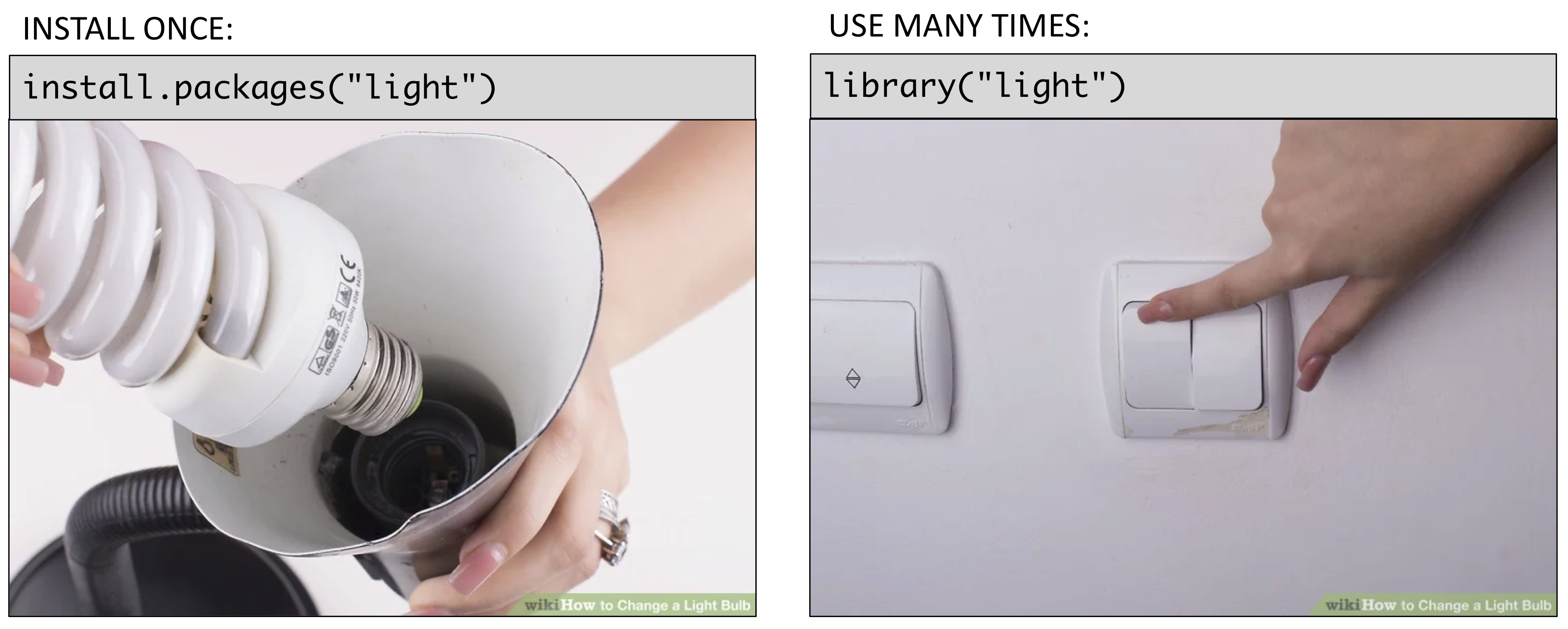
7.2 Using packages
After installing a package, you can’t immediately use the functions
that the package contains. This is because when you start up R only the
“base” functions are loaded. If you want R to also load the functions
inside a package, you have to load that package, which you do
with the library() function. In contrast to the
install.packages() function, you don’t need quotes around
the package name to load it:
library("packagename") # This works
library(packagename)   # This also works
Here’s a helpful image to keep the two ideas of installing vs loading separate:
7.3 Example: wikifacts
As an example, try installing the Wikifacts package, by Keith McNulty:
install.packages("wikifacts") # Remember - you only have to do this once!Now that you have the package installed on your computer, try loading
it using library(wikifacts), then trying using some of it’s
functions:
library(wikifacts) # Load the librarywiki_randomfact()## [1] "Did you know that on June 11 in 1963 – Vietnamese monk Thích Quảng Đức burned himself to death in Saigon to protest the persecution of Buddhists by South Vietnamese President Ngo Dinh Diem's administration. (Courtesy of Wikipedia)"wiki_didyouknow()## [1] "Did you know that Los Angeles was built with the labor of Indigenous Yaangavit people whose village was destroyed to make space for it? (Courtesy of Wikipedia)"In case you’re wondering, the only thing this package does is generate messages containing random facts from Wikipedia.
7.4 Using only some package functions
Sometimes you may only want to use a single function from a library without having to load the whole thing. To do so, use this recipe:
packagename::functionname()
Here I use the name of the package followed by
:: to tell R that I’m looking for a function that is in
that package. For example, if I didn’t want to load the whole
wikifacts library but still wanted to use the
wiki_randomfact() function, I could do this:
wikifacts::wiki_randomfact()## [1] "Here's some news from 04 November 2022. In baseball, the Orix Buffaloes defeat the Tokyo Yakult Swallows to win the Japan Series. (Courtesy of Wikipedia)"Where this is particularly handy is when two packages have a function
with the same name. If you load both library, R might not know which
function to use. In those cases, it’s best to also provide the
package name. For example, let’s say there was a
package called apples and another called
bananas, and each had a function named
fruitName(). If I wanted to use each of them in my code, I
would need to specify the package names like this:
apples::fruitName()
bananas::fruitName()
8 Staying organized
8.1 The history pane
R keeps track of your “command history.” If you click on the console and hit the “up” key, the R console will show you the most recent command that you’ve typed. Hit it again, and it will show you the command before that, and so on.
The second way to get access to your command history is to look at the history panel in Rstudio. On the upper right hand side of the Rstudio window you’ll see a tab labeled “History.” Click on that and you’ll see a list of all your recent commands displayed in that panel. It should look something like this:
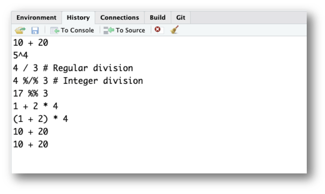
If you double click on one of the commands, it will be copied to the R console.
8.2 Working directory
Any process running on your computer has a notion of its “working directory”. In R, this is where R will look for files you ask it to load. It’s also where any files you write to disk will go.
You can explicitly check your working directory with:
getwd()It is also displayed at the top of the RStudio console.
As a beginning R user, it’s OK let your home directory or any other weird directory on your computer be R’s working directory. Very soon, I urge you to evolve to the next level, where you organize your analytical projects into directories and, when working on project A, set R’s working directory to the associated directory.
Although I do not recommend it, in case you’re curious, you can set R’s working directory at the command line like so:
setwd("~/myCoolProject")Although I do not recommend it, you can also use RStudio’s Files pane to navigate to a directory and then set it as working directory from the menu:
Session > Set Working Directory > To Files Pane Location.
You’ll see even more options there). Or within the Files pane, choose More and Set As Working Directory.
But there’s a better way. A way that also puts you on the path to managing your R work like an expert.
8.3 RStudio projects
Keeping all the files associated with a project organized together – input data, R scripts, analytical results, figures – is such a wise and common practice that RStudio has built-in support for this via its projects.
Let’s make one for practice. Do this:
File > New Project ….
You should see the following pane:
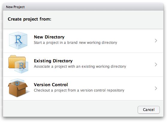
Choose “New Directory”. The directory name you choose here will be the project name. Call it whatever you want. RStudio will create a folder with that name to put all your project files.
As a demo, I created a project on my Desktop called “demo”. RStudio created a new project called “demo”, and in this folder there is a file called “demo.Rproj”. If I double-click on this file, RStudio will open up, and my working directory will be automatically set to this folder! You can double check this by typing:
getwd()8.4 Save your code in .R Files
It is traditional to save R scripts with a .R or
.r suffix. Any code you wish to re-run again later should
be saved in this way and stored within your project folder. For example,
if you wanted to run some of the code in this tutorial, open a new
.R file and save it to your R project folder. Do this:
File > New File > R Script
Then type in some code to re-run it again later. For example:
3 + 4
3 + "4"
x <- 2
x
x <- 42
x
this_is_a_long_name <- 2.5
cases_matter <- 2
Cases_matter <- 3
cases_matter
Cases_matter
cat("Hello world!")
3        + 4
            3   + 4
2 + 2 # I'm adding two numbers
getwd()
Then save this new R script with some name. Do this:
File > Save
I called the file “tutorial.R” and saved it in my R project folder called “demo”.
Now when I open the “demo.Rproj” file, I see in my files pane the “tutorial.R” code script. I can click on that file and continue editing it!
I can also run any line in the script by typing “Command + Enter” (Mac) or “Control + Enter” (Windows).
Page sources:
Some content on this page has been modified from other courses, including:
- “Case” art by Allison Horst
- Danielle Navarro’s book “Learning Statistics With R”
- Danielle Navarro’s website “R for Psychological Science”
- Jenny Bryan’s STAT 545 Course
- Modern Dive, by Chester Ismay & Albert Y. Kim
- RStudio primers
- Xiao Ping Song’s Intro2R crash course
For a more precise statement, see the operator precedence for R.↩︎